Research: Machine learning research
Multimodal smart-home activity recognition
Sparse motion and door sensor logs turned into sequence, text, raster and graph views of the same event window, with the preprocessing, experiment and inspection tooling to evaluate them across four homes.
- Context
- M.S. thesis, University of Georgia
- Technologies
- Python
- PyTorch
- PyTorch Geometric
- Transformers
- CNNs
- Graph neural networks
- CASAS datasets
- YAML metadata
Overview
A smart home can recognise what a resident is doing without cameras. The only input is a log of ambient sensor events, such as a kitchen motion sensor turning on or the front door opening.
My thesis converts that sparse log into four synchronized views of the same short window of events: a sequence, a deterministic text summary, a raster image on the floor plan, and a graph. A matching neural encoder reads each view, a fusion model combines them, and the experiments test when the combination helps. These are four representations of one stream, not four separate sensor feeds.
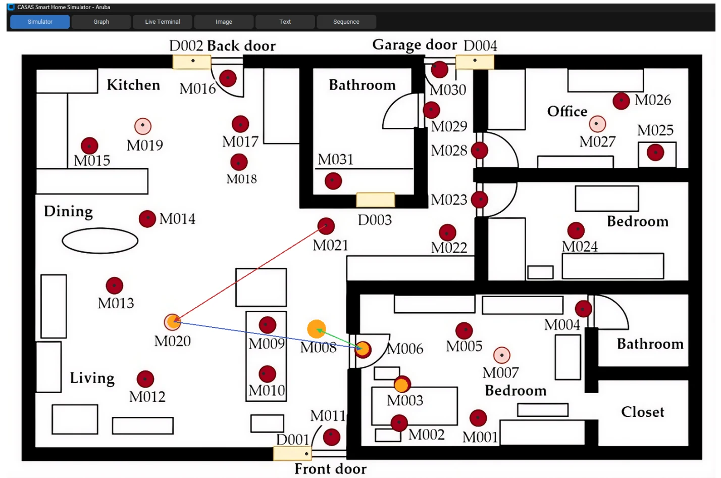
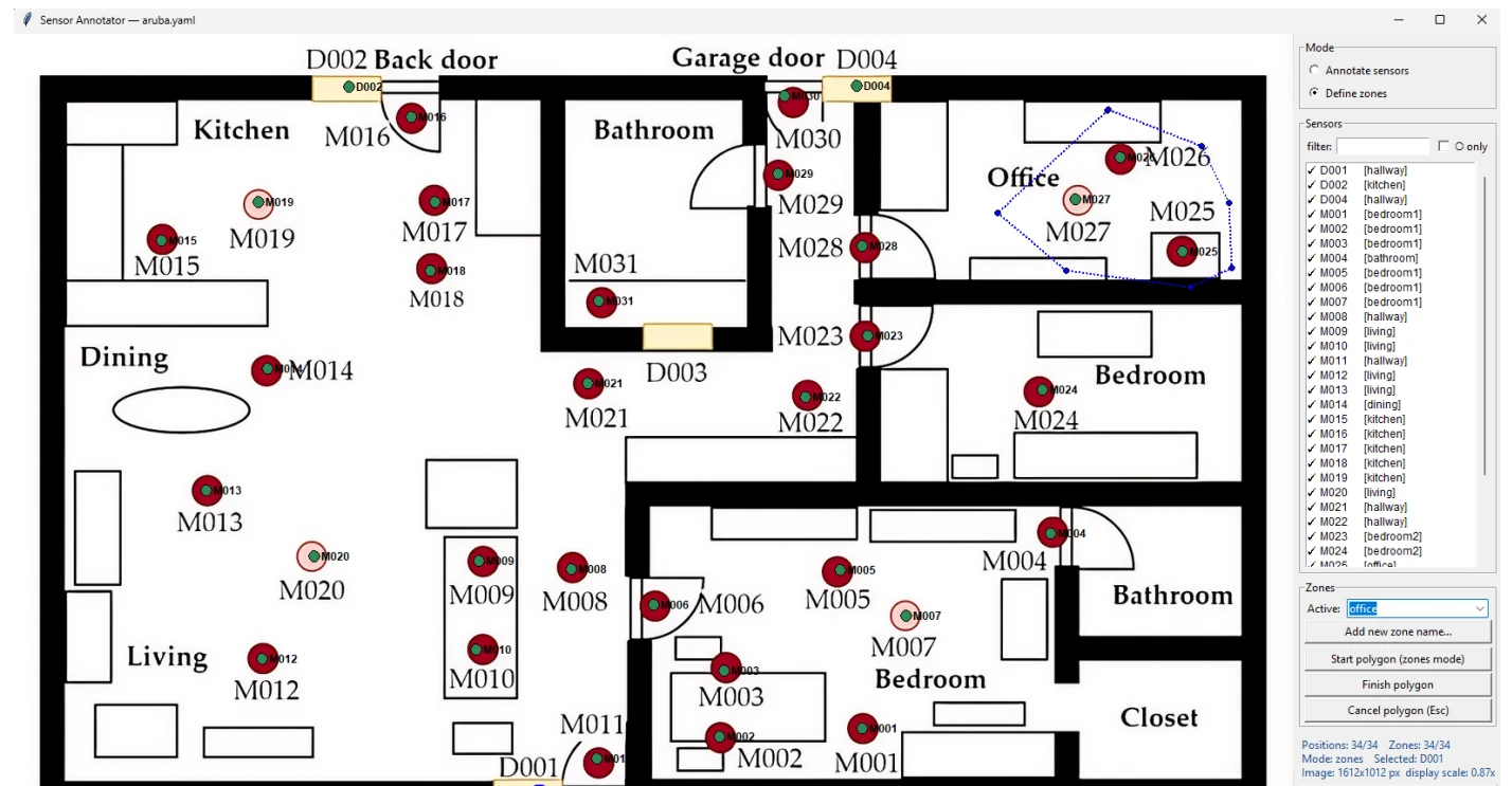
Around the model I built the tools needed to run and trust the experiments: a single experiment-intent configuration, a playback simulator and a sensor and zone annotation tool.
My role and team
- My contribution
- Thesis author. I built and ran the preprocessing, four-view pipeline, multimodal model, experiment tooling and evaluation described here.
- Team context
- Individual thesis work in Fei Dou's research group at the University of Georgia. A lab colleague helped set up the baseline experiments, and one baseline (SICA) comes from my advisor's group.
Problem and constraints
Four things make this problem harder than it looks.
- Ambiguity. The same kitchen sensors can mean cooking, eating or taking medicine.
- Class imbalance. Common background activity far outnumbers rare activities, so accuracy and weighted-F1 can look strong while rare activities fail.
- Different homes. Sensor layouts and activity vocabularies differ: Cairo has no door sensors, Kyoto has 55 sensors, and label sets range from seven to ten classes.
- Irregular data. Events arrive when the resident moves, not on a fixed clock, so a window of events can span seconds or many minutes.
- Fair comparison. Baselines and the proposed model must be trained and tested on exactly the same samples.
Architecture and data flow
The pipeline is driven by per-house metadata, so the same code runs on every house.
Sensor log
- Timestamped motion and door events
- One house, one metadata file
Event windows
- 30 events, stride 15
- Windows never mix activity labels
Four derived views
- Sequence of event features
- Deterministic text summary
- Floor-plan raster image
- Event graph
Encoders
- Transformer
- Transformer
- CNN
- Graph network
Fusion and classifier
- Fusion transformer
- Auxiliary heads per view
- Activity label
Parse and validate
A YAML file per house lists accepted sensors, state mapping, the floor plan, sensor pixel positions, zones and label remaps. Each raw row becomes a timestamp, sensor, state and label record. Unknown sensors and invalid labels are dropped.
Cut event windows
Contiguous runs with the same activity label are cut into 30-event windows with a stride of 15. Runs shorter than 30 events are padded from same-label neighbours so a window never mixes labels.
Derive four views
Sequence: seven feature groups per event, including cyclic time-of-day and log-scaled gaps. Text: a deterministic summary of zones, pace, time of day and revisits. Image: a 96 by 96 raster on the floor plan with six base channels plus one per zone. Graph: event nodes and sensor super nodes with sequential, same-sensor, temporal and sensor-link edges.
Encode and fuse
Each view has its own encoder (two transformers, a CNN and a graph network with local message passing and global attention). Embeddings share a 256-dimensional space and enter a fusion transformer. Auxiliary heads per view, per-class ensemble weights and entropy-based confidence gating let each class lean on the views that help it.
Pretrain, then fine-tune
Encoders can be pretrained without labels, treating the four views of one window as positives for each other, plus masked sensor prediction. Fine-tuning starts with frozen encoders, then unfreezes them with separate learning rates.
Implementation decisions
- Event-count windows instead of clock windows
- A fixed number of events keeps the amount of evidence constant while real time varies. Thirty events was the main setting. A 10-event check tested the opposite trade-off.
- Never mix labels inside a window
- The conservative padding policy avoids mixed-label windows. The trade-off is that some short, rare activities contain repeated evidence, so their F1 has to be read together with their support.
- Describe houses in metadata, not in code
- Adding a house means providing an event CSV and a metadata file. The annotation tool writes sensor coordinates and zone assignments directly into that metadata.
- Select checkpoints on validation macro-F1
- Choosing checkpoints by accuracy or weighted-F1 would reward high-support classes. Final predictions are the argmax of the model logits, with no threshold tuning or post-processing.
- Share the same windows across every model
- Segmentation, labelling and the train and test partitions are produced once and reused by the baselines, so differences come from representation and model learning, not sample construction.
- Build inspection tools before trusting numbers
- The simulator replays events over the floor plan and shows each window's four views. It is not used for training. It exists to catch misaligned sensor coordinates, implausible images and labels that disagree with the visible event trace.
- One experiment-intent file
- A compact file names the house, window size, stride, seeds and run flags. A script expands it into per-house and per-seed configurations, so changing the window size updates dimensions and paths together.
Evaluation protocol
How the numbers below were produced.
- Data: four CASAS houses. Aruba has 34 sensors and 9 classes, Cairo 27 and 7, Kyoto 55 and 7, Milan 31 and 10. An Other class is kept where the house defines one.
- Windows: 30 events with stride 15 for the main results, plus a 10-event, stride-5 robustness check.
- Fairness: a shared first stage produces identical samples and train and test partitions for the proposed model and all baselines.
- Baselines: SICA, CPC, DeepCASAS and DCNN.
- Ablation: all 15 combinations of the four views, per house.
- Seeds and aggregation: seeds 10, 30 and 50, reported as means over the three seeds.
- Metrics: accuracy, weighted-F1 and macro-F1. Weighted-F1 follows the observed class distribution. Macro-F1 gives every class equal weight and exposes minority-class failures. Both are shown here.
Results and context
Best proposed configuration per house, ranked by weighted-F1, next to the strongest selected baseline on the same metric. Main 30-event setting, mean of three seeds.
| House | Best proposed configuration | Weighted-F1 | Macro-F1 | Strongest baseline | Baseline weighted-F1 | Baseline macro-F1 |
|---|---|---|---|---|---|---|
| Aruba | graph + image + sequence | 0.850 | 0.735 | SICA | 0.847 | 0.638 |
| Cairo | graph + text + image | 0.842 | 0.524 | SICA | 0.755 | 0.181 |
| Kyoto | image + text + sequence | 0.843 | 0.766 | SICA | 0.821 | 0.726 |
These describe each house on its own. They are not evidence that a model transfers to an unseen home.
- The best configuration differs by house. That argues for choosing views per house rather than assuming more views always help.
- The metric changes the story. In Aruba, CPC has slightly higher macro-F1 (0.740) than the best proposed configuration (0.735). In Kyoto, graph + text has higher macro-F1 (0.777) than image + text + sequence (0.766). In Cairo, graph + sequence has the highest macro-F1 among proposed models (0.550).
- Cairo shows the widest gap between weighted-F1 (0.842) and macro-F1 (0.524), which points to persistent difficulty with rare activities such as taking medication.
- In the 10-event check, longer windows raised macro-F1 for Aruba (0.533 to 0.735) and Cairo (0.405 to 0.524), while Kyoto was marginally higher with the shorter window (0.774 against 0.766).
- Milan, with ten activity classes, was the hardest house. The all-four-view model was the strongest proposed configuration there by macro-F1. Exact Milan figures are not summarised on this page.
Limitations and lessons
Limitations
- Class spaces differ between houses, so macro-F1 should not be compared across houses.
- Rare-class F1 is statistically fragile. Some activities have little test support and shift with the seed, the day selection and label remapping.
- Models are trained and tested within a house. I did not evaluate transfer to unseen homes or residents, so this work does not show generalisation without retraining.
- The inspection tools were not evaluated in a user study. Their value here is practical: fewer metadata mistakes during experiments.
- Some thesis figures show validation-style diagnostics while the tables report test means across seeds.
What I took from it
- Report macro-F1 and per-class diagnostics next to weighted-F1. In my own results one metric alone would have hidden failures on rare activities.
- Inspection tooling pays for itself early. Looking at windows over the floor plan found problems that would otherwise have shown up as mysteriously weak model scores.
- Deriving every path and dimension from one intent file removed a whole class of configuration mistakes.
Artifacts
The thesis PDF and code are not linked from this site yet. The interactive demo is an educational illustration built with synthetic data, not the research code.